试验设计与数据分析
  1. 试验设计与方差分析
  2. 10  裂区试验设计
  1. 试验设计与方差分析
  2. 10  裂区试验设计

10  裂区试验设计

  • 主页

  • 试验设计概述
    • 1  试验设计基础

  • R语言基础
    • 2  Rstudio环境配置
    • 3  数据类型与基本语法

  • Tidyverse学习
    • 4  tidyverse简介
    • 5  数据读取与导出
    • 6  ggplot2
    • 7  grid系统

  • 回归与拟合
    • 8  线性和非线性拟合

  • 试验设计与方差分析
    • 9  随机区组试验设计
    • 10  裂区试验设计

  • 高级统计分析
    • 11  通径分析
    • 12  随机森林回归
    • 13  主成分分析(PCA)
    • 14  冗余分析
    • 15  结构方程模型
    • 16  弦图(Chord diagram)
    • 17  Meta分析

  • 关于

页内导航

  • 10.1 加载环境与数据准备
    • 10.1.1 安装包检测并自动安装(必须联网)
    • 10.1.2 加载R必备包
    • 10.1.3 试验数据读取
  • 10.2 试验数据检测
  • 10.3 方差分析
  • 10.4 事后均值对比
    • 10.4.1 定义HSD结果提取函数
    • 10.4.2 对第1因子进行HSD均值检测
    • 10.4.3 对第2因子进行HSD均值检测
    • 10.4.4 对交互因子进行HSD均值检测
  • 10.5 出图
    • 10.5.1 设置试验因子各水平排序
    • 10.5.2 第1因子灌溉模式不同水平均值对比
    • 10.5.3 第2因子生物炭不同水平均值对比
    • 10.5.4 交互因子不同处理间平均值对比
    • 10.5.5 合成并出图

10.1 加载环境与数据准备

10.1.1 安装包检测并自动安装(必须联网)

pkgs <- c("tidyverse","agricolae","here","knitr","latex2exp","cowplot")                   
not_installed <- pkgs[!(pkgs %in% installed.packages()[ , "Package"])]   
if(length(not_installed)) install.packages(not_installed)  

10.1.2 加载R必备包

library(tidyverse)
library(agricolae)
library(here)
library(knitr)
library(latex2exp)
library(cowplot)
options(digits = 4)

10.1.3 试验数据读取

dt <- readxl::read_excel(here("RES/dataset/产量干物质.xlsx"),
                         sheet = "干物质",
                         skip = 2) 
dt <- dt %>% filter(Sampling == 1) %>% select(-Sampling)
dt
表 10.1 试验数据集
PlotID Rep Irrigation Biochar Grainyield DMA
1 R1 CF B0 8.578 18.75
2 R1 CF B20 8.653 16.98
3 R1 CF B20M 7.852 15.79
4 R1 AWD B0 7.811 16.16
5 R1 AWD B20 8.794 17.56
6 R1 AWD B20M 6.509 14.05
7 R2 CF B0 7.474 16.93
8 R2 CF B20 7.806 14.21
9 R2 CF B20M 7.386 15.71
10 R2 AWD B0 6.956 14.58
11 R2 AWD B20 6.953 13.01
12 R2 AWD B20M 7.878 16.60
13 R3 CF B0 6.346 12.45
14 R3 CF B20 8.881 18.98
15 R3 CF B20M 8.157 17.87
16 R3 AWD B0 9.809 19.93
17 R3 AWD B20 7.234 13.80
18 R3 AWD B20M 6.190 11.49

10.2 试验数据检测

详细过程见Section 9.2部分。

10.3 方差分析

由此可见,试验数据满足正态和方差齐次性,可正常进行方差分析。

以表 15.1数据集为例,采用随机区组试验设计模型对试验数据进行方差分析,结果如表 10.2。

response <- dt$Grainyield
ANOVA <- aov(response ~ Rep + Irrigation * Biochar + Error(Rep/Irrigation), data = dt) %>%
  summary()
ANOVA <- pmap_df(list(data=ANOVA,name=names(ANOVA)),~.x[[1]],.id = "error") %>% 
  mutate(error=error %>% as.character())

ANOVA %>% select(-error) %>%
  kable(digits=3)
表 10.2 随机区组试验方差分析表
Df Sum Sq Mean Sq F value Pr(>F)
Rep 2 1.177 0.589 NA NA
Irrigation 1 0.499 0.499 3.579 0.199
Residuals 2 0.279 0.140 NA NA
Biochar 2 1.650 0.825 0.671 0.538
Irrigation:Biochar 2 2.542 1.271 1.033 0.399
Residuals 8 9.841 1.230 NA NA

有的学者可能对方差贡献率感兴趣,利用各因子及交互效应等平方和数据,可进一步得到各因子和交互效应贡献率情况,如表 10.3。

ANOVA %>%  select(-error) %>%
  mutate(Contri=`Sum Sq`/sum(`Sum Sq`)*100) %>%
  kable(digits = 3)
表 10.3 方差分析+方差贡献率
Df Sum Sq Mean Sq F value Pr(>F) Contri
Rep 2 1.177 0.589 NA NA 7.363
Irrigation 1 0.499 0.499 3.579 0.199 3.123
Residuals 2 0.279 0.140 NA NA 1.745
Biochar 2 1.650 0.825 0.671 0.538 10.321
Irrigation:Biochar 2 2.542 1.271 1.033 0.399 15.899
Residuals 8 9.841 1.230 NA NA 61.548

10.4 事后均值对比

10.4.1 定义HSD结果提取函数

getHSD <- function(hsd){
  merge(x=hsd$means %>% select(std),
        y=hsd$groups,
        by="row.names") %>% 
    rename(trt=Row.names)
}

10.4.2 对第1因子进行HSD均值检测

# Irrigation 主区误差项
DFerror1 <- ANOVA %>% filter(error=="Error: Rep:Irrigation" & is.na(`F value`)) %>% getElement("Df")
MSerror1 <- ANOVA %>% filter(error=="Error: Rep:Irrigation" & is.na(`F value`)) %>% getElement("Mean Sq")

# Biochar和交互效应共一个误差项
DFerror2 <- ANOVA %>% filter(error=="Error: Within" & is.na(`F value`)) %>% getElement("Df")
MSerror2 <- ANOVA %>% filter(error=="Error: Within" & is.na(`F value`)) %>% getElement("Mean Sq")

means <- dt$Grainyield
hsd.Irrigation <- HSD.test(
  means,
  trt = dt$Irrigation,
  DFerror = DFerror1,
  MSerror = MSerror1
) %>%
  getHSD() %>% select(trt, means, std, groups)

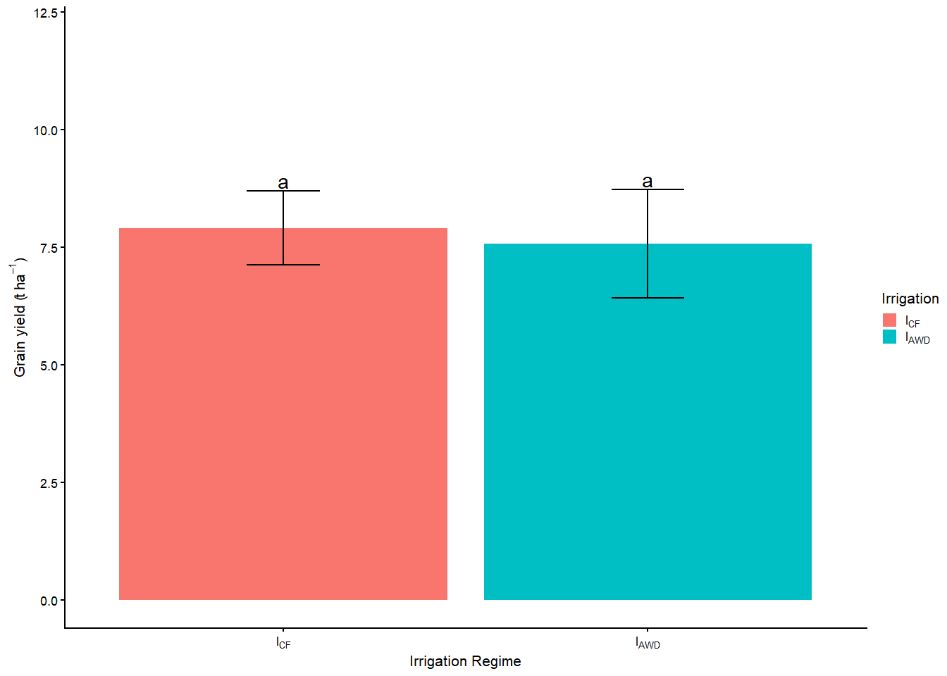
hsd.Irrigation %>%  kable(digits=3)
表 10.4 不同灌溉模式下产量均值对比结果
trt means std groups
AWD 7.570 1.149 a
CF 7.904 0.785 a

10.4.3 对第2因子进行HSD均值检测

hsd.Biochar <- HSD.test(means,
                        trt = dt$Biochar,
                        DFerror = DFerror2,
                        MSerror = MSerror2) %>%
  getHSD() %>% select(trt, means, std, groups)

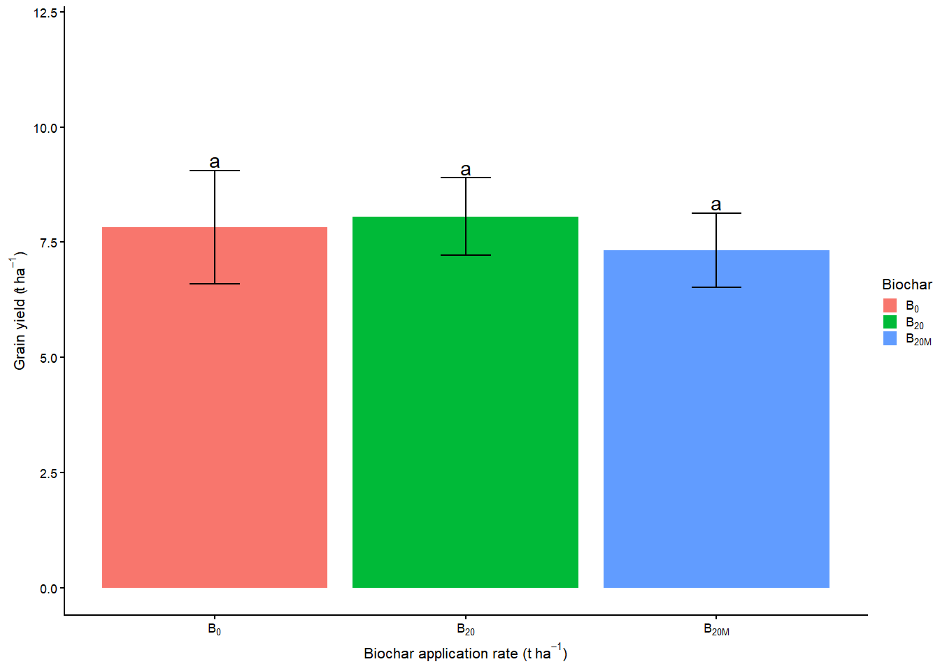
hsd.Biochar %>%  kable(digits=3)
表 10.5 不同生物炭水平下产量均值对比结果
trt means std groups
B0 7.829 1.230 a
B20 8.053 0.841 a
B20M 7.329 0.804 a

10.4.4 对交互因子进行HSD均值检测

hsd.Interaction <- HSD.test(
  means,
  trt = interaction(dt$Irrigation, dt$Biochar),
  DFerror = DFerror2,
  MSerror = MSerror2
) %>%
  getHSD() %>% select(trt, means, std, groups) %>% separate(col = trt, into =
                                                              c("Irrigation", "Biochar"))

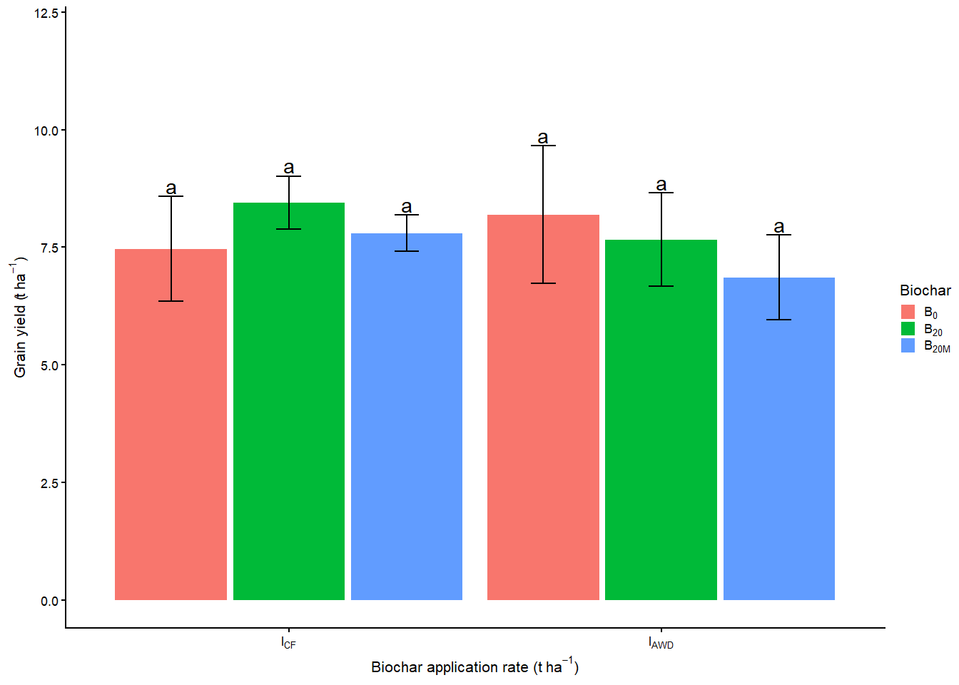
hsd.Interaction%>%  kable(digits=3)
表 10.6 不同灌溉模式和生物炭水平下产量均值对比结果
Irrigation Biochar means std groups
AWD B0 8.192 1.464 a
AWD B20 7.660 0.992 a
AWD B20M 6.859 0.897 a
CF B0 7.466 1.116 a
CF B20 8.446 0.566 a
CF B20M 7.799 0.388 a

10.5 出图

10.5.1 设置试验因子各水平排序

hsd.Irrigation$trt <- hsd.Irrigation$trt %>% fct_relevel("CF", "AWD")
hsd.Biochar$trt <- hsd.Biochar$trt %>% fct_relevel("B0", "B20", "B20M")
hsd.Interaction$Irrigation <-  hsd.Interaction$Irrigation %>% fct_relevel("CF", "AWD")
hsd.Interaction$Biochar <- hsd.Interaction$Biochar %>% fct_relevel("B0", "B20", "B20M")

mylabels.irr <- c(CF = TeX("$I_{CF}$"), AWD = TeX("$I_{AWD}$"))
mylabels.bio <- c(
  B0 = TeX("$B_{0}$"),
  B20 = TeX("$B_{20}$"),
  B20M = TeX("$B_{20M}$")
)

10.5.2 第1因子灌溉模式不同水平均值对比

G.irr <- ggplot(hsd.Irrigation ,aes(x=trt,y=means,fill=trt ))+
  geom_bar(stat="identity")+
  geom_errorbar(aes(ymin=means-std,ymax=means+std),
                width=0.2)+
  geom_text(aes(y=means+std,label=groups),vjust=-0.2)+
  cowplot::theme_cowplot(font_size = 8,line_size = 0.4)+
  scale_fill_discrete(labels=mylabels.irr )+
  scale_x_discrete(labels=mylabels.irr )+
  ylim(0,12)+
  labs(x = "Irrigation Regime",
       y = TeX("Grain yield ($t~ha^{-1}$)"),
       fill = "Irrigation")
G.irr
图 10.1 不同灌溉模式下产量情况

10.5.3 第2因子生物炭不同水平均值对比

G.Bio <- ggplot(hsd.Biochar ,aes(x=trt,y=means,fill=trt ))+
  geom_bar(stat = "identity") +
  geom_errorbar(aes(ymin = means - std, ymax = means + std), width = 0.2) +
  geom_text(aes(y = means + std, label = groups), vjust = -0.2) +
  cowplot::theme_cowplot(font_size = 8, line_size = 0.4) +
  scale_fill_discrete(labels = mylabels.bio) +
  scale_x_discrete(labels = mylabels.bio) +
  ylim(0, 12) +
  labs(
    x = TeX("Biochar application rate ($t~ha^{-1}$)"),
    y = TeX("Grain yield ($t~ha^{-1}$)"),
    fill = "Biochar"
  ) 
G.Bio
图 10.2 不同生物炭水平下产量情况

10.5.4 交互因子不同处理间平均值对比

dod <- position_dodge(width = 0.95)
G.int <- ggplot(hsd.Interaction , aes(x = Irrigation, y = means, fill = Biochar)) +
  geom_bar(stat = "identity", position = dod) +
  geom_errorbar(aes(ymin = means - std, ymax = means + std),
                position = dod,
                width = 0.2) +
  geom_text(aes(y = means + std, label = groups),
            vjust = -0.2,
            position = dod) +
  cowplot::theme_cowplot(font_size = 8, line_size = 0.4) +
  scale_x_discrete(labels = mylabels.irr) +
  scale_fill_discrete(labels = mylabels.bio) +
  ylim(0, 12) +
  labs(
    x = TeX("Biochar application rate ($t~ha^{-1}$)"),
    y = TeX("Grain yield ($t~ha^{-1}$)")
  )
G.int
图 10.3 不同灌溉模式和生物炭水平下产量情况

10.5.5 合成并出图

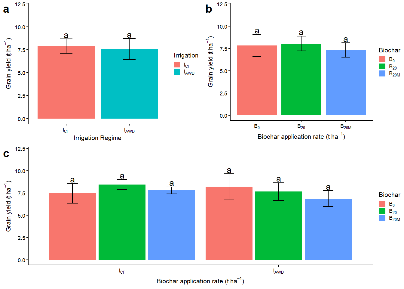
GG <- plot_grid(
  plot_grid(G.irr, G.Bio, nrow = 1, labels = letters),
  G.int,
  nrow = 2,
  labels = c("", "c")
)
GG
图 10.4 主效应和交互效应
9  随机区组试验设计
Source Code
# 裂区试验设计

## 加载环境与数据准备

### 安装包检测并自动安装(必须联网)

```{r}
pkgs <- c("tidyverse","agricolae","here","knitr","latex2exp","cowplot")                   
not_installed <- pkgs[!(pkgs %in% installed.packages()[ , "Package"])]   
if(length(not_installed)) install.packages(not_installed)  
```

### 加载R必备包

```{r}
#| warning: false
#| label: loadingPackage
library(tidyverse)
library(agricolae)
library(here)
library(knitr)
library(latex2exp)
library(cowplot)
options(digits = 4)
```

### 试验数据读取

```{r}
#| label: tbl-dataset
#| tbl-cap: "试验数据集"

dt <- readxl::read_excel(here("RES/dataset/产量干物质.xlsx"),
                         sheet = "干物质",
                         skip = 2) 
dt <- dt %>% filter(Sampling == 1) %>% select(-Sampling)
dt
```

## 试验数据检测
详细过程见[@sec-datatest]部分。

## 方差分析
由此可见,试验数据满足正态和方差齐次性,可正常进行方差分析。

以[@tbl-dataset]数据集为例,采用随机区组试验设计模型对试验数据进行方差分析,结果如[@tbl-ANOVA]。

```{r}
#| label: tbl-ANOVA
#| tbl-cap: "随机区组试验方差分析表"
response <- dt$Grainyield
ANOVA <- aov(response ~ Rep + Irrigation * Biochar + Error(Rep/Irrigation), data = dt) %>%
  summary()
ANOVA <- pmap_df(list(data=ANOVA,name=names(ANOVA)),~.x[[1]],.id = "error") %>% 
  mutate(error=error %>% as.character())

ANOVA %>% select(-error) %>%
  kable(digits=3)
```
有的学者可能对方差贡献率感兴趣,利用各因子及交互效应等平方和数据,可进一步得到各因子和交互效应贡献率情况,如[@tbl-ANOVA-Contribution]。

```{r}
#| label: tbl-ANOVA-Contribution
#| tbl-cap: "方差分析+方差贡献率"
ANOVA %>%  select(-error) %>%
  mutate(Contri=`Sum Sq`/sum(`Sum Sq`)*100) %>%
  kable(digits = 3)
```

## 事后均值对比

### 定义HSD结果提取函数
```{r}
getHSD <- function(hsd){
  merge(x=hsd$means %>% select(std),
        y=hsd$groups,
        by="row.names") %>% 
    rename(trt=Row.names)
}
```
### 对第1因子进行HSD均值检测

```{r}
#| label: tbl-hsd-irrigation
#| tbl-cap: "不同灌溉模式下产量均值对比结果"

# Irrigation 主区误差项
DFerror1 <- ANOVA %>% filter(error=="Error: Rep:Irrigation" & is.na(`F value`)) %>% getElement("Df")
MSerror1 <- ANOVA %>% filter(error=="Error: Rep:Irrigation" & is.na(`F value`)) %>% getElement("Mean Sq")

# Biochar和交互效应共一个误差项
DFerror2 <- ANOVA %>% filter(error=="Error: Within" & is.na(`F value`)) %>% getElement("Df")
MSerror2 <- ANOVA %>% filter(error=="Error: Within" & is.na(`F value`)) %>% getElement("Mean Sq")

means <- dt$Grainyield
hsd.Irrigation <- HSD.test(
  means,
  trt = dt$Irrigation,
  DFerror = DFerror1,
  MSerror = MSerror1
) %>%
  getHSD() %>% select(trt, means, std, groups)

hsd.Irrigation %>%  kable(digits=3)
```


### 对第2因子进行HSD均值检测

```{r}
#| label: tbl-hsd-biochar
#| tbl-cap: "不同生物炭水平下产量均值对比结果"
#| 
hsd.Biochar <- HSD.test(means,
                        trt = dt$Biochar,
                        DFerror = DFerror2,
                        MSerror = MSerror2) %>%
  getHSD() %>% select(trt, means, std, groups)

hsd.Biochar %>%  kable(digits=3)
```

### 对交互因子进行HSD均值检测

```{r}
#| label: tbl-hsd-interaction
#| tbl-cap: "不同灌溉模式和生物炭水平下产量均值对比结果"
#| 
hsd.Interaction <- HSD.test(
  means,
  trt = interaction(dt$Irrigation, dt$Biochar),
  DFerror = DFerror2,
  MSerror = MSerror2
) %>%
  getHSD() %>% select(trt, means, std, groups) %>% separate(col = trt, into =
                                                              c("Irrigation", "Biochar"))

hsd.Interaction%>%  kable(digits=3)
```

## 出图

### 设置试验因子各水平排序

```{r}
hsd.Irrigation$trt <- hsd.Irrigation$trt %>% fct_relevel("CF", "AWD")
hsd.Biochar$trt <- hsd.Biochar$trt %>% fct_relevel("B0", "B20", "B20M")
hsd.Interaction$Irrigation <-  hsd.Interaction$Irrigation %>% fct_relevel("CF", "AWD")
hsd.Interaction$Biochar <- hsd.Interaction$Biochar %>% fct_relevel("B0", "B20", "B20M")

mylabels.irr <- c(CF = TeX("$I_{CF}$"), AWD = TeX("$I_{AWD}$"))
mylabels.bio <- c(
  B0 = TeX("$B_{0}$"),
  B20 = TeX("$B_{20}$"),
  B20M = TeX("$B_{20M}$")
)
```

### 第1因子灌溉模式不同水平均值对比
```{r}
#| label: fig-ggplot-irrigation
#| fig-cap: "不同灌溉模式下产量情况"
G.irr <- ggplot(hsd.Irrigation ,aes(x=trt,y=means,fill=trt ))+
  geom_bar(stat="identity")+
  geom_errorbar(aes(ymin=means-std,ymax=means+std),
                width=0.2)+
  geom_text(aes(y=means+std,label=groups),vjust=-0.2)+
  cowplot::theme_cowplot(font_size = 8,line_size = 0.4)+
  scale_fill_discrete(labels=mylabels.irr )+
  scale_x_discrete(labels=mylabels.irr )+
  ylim(0,12)+
  labs(x = "Irrigation Regime",
       y = TeX("Grain yield ($t~ha^{-1}$)"),
       fill = "Irrigation")
G.irr
```


### 第2因子生物炭不同水平均值对比
```{r}
#| label: fig-ggplot-biochar
#| fig-cap: "不同生物炭水平下产量情况"
G.Bio <- ggplot(hsd.Biochar ,aes(x=trt,y=means,fill=trt ))+
  geom_bar(stat = "identity") +
  geom_errorbar(aes(ymin = means - std, ymax = means + std), width = 0.2) +
  geom_text(aes(y = means + std, label = groups), vjust = -0.2) +
  cowplot::theme_cowplot(font_size = 8, line_size = 0.4) +
  scale_fill_discrete(labels = mylabels.bio) +
  scale_x_discrete(labels = mylabels.bio) +
  ylim(0, 12) +
  labs(
    x = TeX("Biochar application rate ($t~ha^{-1}$)"),
    y = TeX("Grain yield ($t~ha^{-1}$)"),
    fill = "Biochar"
  ) 
G.Bio
```

### 交互因子不同处理间平均值对比
```{r}
#| label: fig-ggplot-interaction
#| fig-cap: "不同灌溉模式和生物炭水平下产量情况"
dod <- position_dodge(width = 0.95)
G.int <- ggplot(hsd.Interaction , aes(x = Irrigation, y = means, fill = Biochar)) +
  geom_bar(stat = "identity", position = dod) +
  geom_errorbar(aes(ymin = means - std, ymax = means + std),
                position = dod,
                width = 0.2) +
  geom_text(aes(y = means + std, label = groups),
            vjust = -0.2,
            position = dod) +
  cowplot::theme_cowplot(font_size = 8, line_size = 0.4) +
  scale_x_discrete(labels = mylabels.irr) +
  scale_fill_discrete(labels = mylabels.bio) +
  ylim(0, 12) +
  labs(
    x = TeX("Biochar application rate ($t~ha^{-1}$)"),
    y = TeX("Grain yield ($t~ha^{-1}$)")
  )
G.int
```

### 合成并出图
```{r}
#| label: fig-ggplot-merge
#| fig-cap: "主效应和交互效应"

GG <- plot_grid(
  plot_grid(G.irr, G.Bio, nrow = 1, labels = letters),
  G.int,
  nrow = 2,
  labels = c("", "c")
)
GG
```
 

Copyright 2025, Taotao Chen