library(randomForest) # 进行随机森林回归
library(datasets) # 数据集
library(tidyverse) # 数据整理、绘图
library(rfPermute) # 检验变量显著性
library(A3) # 检验模型显著性利用R实现随机森林回归(Random Forest Regression),同时计算模型和变量显著性,绘制带有显著性标注的变量重要性条形图。
12.1 加载工具包
12.2 数据整理
以datasets包自带的airquality数据集为例,首先剔除数据中的空白和无效记录,筛选后的数据集 表 15.1 所示。
data("airquality")
dat <- na.omit(airquality)
dat %>% kableExtra::kable()| Ozone | Solar.R | Wind | Temp | Month | Day | |
|---|---|---|---|---|---|---|
| 1 | 41 | 190 | 7.4 | 67 | 5 | 1 |
| 2 | 36 | 118 | 8.0 | 72 | 5 | 2 |
| 3 | 12 | 149 | 12.6 | 74 | 5 | 3 |
| 4 | 18 | 313 | 11.5 | 62 | 5 | 4 |
| 7 | 23 | 299 | 8.6 | 65 | 5 | 7 |
| 8 | 19 | 99 | 13.8 | 59 | 5 | 8 |
| 9 | 8 | 19 | 20.1 | 61 | 5 | 9 |
| 12 | 16 | 256 | 9.7 | 69 | 5 | 12 |
| 13 | 11 | 290 | 9.2 | 66 | 5 | 13 |
| 14 | 14 | 274 | 10.9 | 68 | 5 | 14 |
| 15 | 18 | 65 | 13.2 | 58 | 5 | 15 |
| 16 | 14 | 334 | 11.5 | 64 | 5 | 16 |
| 17 | 34 | 307 | 12.0 | 66 | 5 | 17 |
| 18 | 6 | 78 | 18.4 | 57 | 5 | 18 |
| 19 | 30 | 322 | 11.5 | 68 | 5 | 19 |
| 20 | 11 | 44 | 9.7 | 62 | 5 | 20 |
| 21 | 1 | 8 | 9.7 | 59 | 5 | 21 |
| 22 | 11 | 320 | 16.6 | 73 | 5 | 22 |
| 23 | 4 | 25 | 9.7 | 61 | 5 | 23 |
| 24 | 32 | 92 | 12.0 | 61 | 5 | 24 |
| 28 | 23 | 13 | 12.0 | 67 | 5 | 28 |
| 29 | 45 | 252 | 14.9 | 81 | 5 | 29 |
| 30 | 115 | 223 | 5.7 | 79 | 5 | 30 |
| 31 | 37 | 279 | 7.4 | 76 | 5 | 31 |
| 38 | 29 | 127 | 9.7 | 82 | 6 | 7 |
| 40 | 71 | 291 | 13.8 | 90 | 6 | 9 |
| 41 | 39 | 323 | 11.5 | 87 | 6 | 10 |
| 44 | 23 | 148 | 8.0 | 82 | 6 | 13 |
| 47 | 21 | 191 | 14.9 | 77 | 6 | 16 |
| 48 | 37 | 284 | 20.7 | 72 | 6 | 17 |
| 49 | 20 | 37 | 9.2 | 65 | 6 | 18 |
| 50 | 12 | 120 | 11.5 | 73 | 6 | 19 |
| 51 | 13 | 137 | 10.3 | 76 | 6 | 20 |
| 62 | 135 | 269 | 4.1 | 84 | 7 | 1 |
| 63 | 49 | 248 | 9.2 | 85 | 7 | 2 |
| 64 | 32 | 236 | 9.2 | 81 | 7 | 3 |
| 66 | 64 | 175 | 4.6 | 83 | 7 | 5 |
| 67 | 40 | 314 | 10.9 | 83 | 7 | 6 |
| 68 | 77 | 276 | 5.1 | 88 | 7 | 7 |
| 69 | 97 | 267 | 6.3 | 92 | 7 | 8 |
| 70 | 97 | 272 | 5.7 | 92 | 7 | 9 |
| 71 | 85 | 175 | 7.4 | 89 | 7 | 10 |
| 73 | 10 | 264 | 14.3 | 73 | 7 | 12 |
| 74 | 27 | 175 | 14.9 | 81 | 7 | 13 |
| 76 | 7 | 48 | 14.3 | 80 | 7 | 15 |
| 77 | 48 | 260 | 6.9 | 81 | 7 | 16 |
| 78 | 35 | 274 | 10.3 | 82 | 7 | 17 |
| 79 | 61 | 285 | 6.3 | 84 | 7 | 18 |
| 80 | 79 | 187 | 5.1 | 87 | 7 | 19 |
| 81 | 63 | 220 | 11.5 | 85 | 7 | 20 |
| 82 | 16 | 7 | 6.9 | 74 | 7 | 21 |
| 85 | 80 | 294 | 8.6 | 86 | 7 | 24 |
| 86 | 108 | 223 | 8.0 | 85 | 7 | 25 |
| 87 | 20 | 81 | 8.6 | 82 | 7 | 26 |
| 88 | 52 | 82 | 12.0 | 86 | 7 | 27 |
| 89 | 82 | 213 | 7.4 | 88 | 7 | 28 |
| 90 | 50 | 275 | 7.4 | 86 | 7 | 29 |
| 91 | 64 | 253 | 7.4 | 83 | 7 | 30 |
| 92 | 59 | 254 | 9.2 | 81 | 7 | 31 |
| 93 | 39 | 83 | 6.9 | 81 | 8 | 1 |
| 94 | 9 | 24 | 13.8 | 81 | 8 | 2 |
| 95 | 16 | 77 | 7.4 | 82 | 8 | 3 |
| 99 | 122 | 255 | 4.0 | 89 | 8 | 7 |
| 100 | 89 | 229 | 10.3 | 90 | 8 | 8 |
| 101 | 110 | 207 | 8.0 | 90 | 8 | 9 |
| 104 | 44 | 192 | 11.5 | 86 | 8 | 12 |
| 105 | 28 | 273 | 11.5 | 82 | 8 | 13 |
| 106 | 65 | 157 | 9.7 | 80 | 8 | 14 |
| 108 | 22 | 71 | 10.3 | 77 | 8 | 16 |
| 109 | 59 | 51 | 6.3 | 79 | 8 | 17 |
| 110 | 23 | 115 | 7.4 | 76 | 8 | 18 |
| 111 | 31 | 244 | 10.9 | 78 | 8 | 19 |
| 112 | 44 | 190 | 10.3 | 78 | 8 | 20 |
| 113 | 21 | 259 | 15.5 | 77 | 8 | 21 |
| 114 | 9 | 36 | 14.3 | 72 | 8 | 22 |
| 116 | 45 | 212 | 9.7 | 79 | 8 | 24 |
| 117 | 168 | 238 | 3.4 | 81 | 8 | 25 |
| 118 | 73 | 215 | 8.0 | 86 | 8 | 26 |
| 120 | 76 | 203 | 9.7 | 97 | 8 | 28 |
| 121 | 118 | 225 | 2.3 | 94 | 8 | 29 |
| 122 | 84 | 237 | 6.3 | 96 | 8 | 30 |
| 123 | 85 | 188 | 6.3 | 94 | 8 | 31 |
| 124 | 96 | 167 | 6.9 | 91 | 9 | 1 |
| 125 | 78 | 197 | 5.1 | 92 | 9 | 2 |
| 126 | 73 | 183 | 2.8 | 93 | 9 | 3 |
| 127 | 91 | 189 | 4.6 | 93 | 9 | 4 |
| 128 | 47 | 95 | 7.4 | 87 | 9 | 5 |
| 129 | 32 | 92 | 15.5 | 84 | 9 | 6 |
| 130 | 20 | 252 | 10.9 | 80 | 9 | 7 |
| 131 | 23 | 220 | 10.3 | 78 | 9 | 8 |
| 132 | 21 | 230 | 10.9 | 75 | 9 | 9 |
| 133 | 24 | 259 | 9.7 | 73 | 9 | 10 |
| 134 | 44 | 236 | 14.9 | 81 | 9 | 11 |
| 135 | 21 | 259 | 15.5 | 76 | 9 | 12 |
| 136 | 28 | 238 | 6.3 | 77 | 9 | 13 |
| 137 | 9 | 24 | 10.9 | 71 | 9 | 14 |
| 138 | 13 | 112 | 11.5 | 71 | 9 | 15 |
| 139 | 46 | 237 | 6.9 | 78 | 9 | 16 |
| 140 | 18 | 224 | 13.8 | 67 | 9 | 17 |
| 141 | 13 | 27 | 10.3 | 76 | 9 | 18 |
| 142 | 24 | 238 | 10.3 | 68 | 9 | 19 |
| 143 | 16 | 201 | 8.0 | 82 | 9 | 20 |
| 144 | 13 | 238 | 12.6 | 64 | 9 | 21 |
| 145 | 23 | 14 | 9.2 | 71 | 9 | 22 |
| 146 | 36 | 139 | 10.3 | 81 | 9 | 23 |
| 147 | 7 | 49 | 10.3 | 69 | 9 | 24 |
| 148 | 14 | 20 | 16.6 | 63 | 9 | 25 |
| 149 | 30 | 193 | 6.9 | 70 | 9 | 26 |
| 151 | 14 | 191 | 14.3 | 75 | 9 | 28 |
| 152 | 18 | 131 | 8.0 | 76 | 9 | 29 |
| 153 | 20 | 223 | 11.5 | 68 | 9 | 30 |
12.3 数据分析
分别采用randomForest包和rfPermute包进行说明。
12.3.1 采用randomForest包
直接采用randomForest包进行数据分析
set.seed(20241102)
rf <- randomForest(Ozone~Solar.R+Wind+Temp, data = dat,  importance=TRUE, ntree=500)
print(rf)
Call:
 randomForest(formula = Ozone ~ Solar.R + Wind + Temp, data = dat,      importance = TRUE, ntree = 500)
               Type of random forest: regression
                     Number of trees: 500
No. of variables tried at each split: 1

          Mean of squared residuals: 301.2151
                    % Var explained: 72.55
由上述结果可知,随机森林生成了500个树,每个节点随机抽取1个变量进行模型拟合。拟合后模型可以解释72.55%的变异。进一步提取随机森林回归贡献率,结果如 表 12.2 所示。
imp <- importance(rf,scale = TRUE)
imp %>% kableExtra::kable()| %IncMSE | IncNodePurity | |
|---|---|---|
| Solar.R | 14.35751 | 23417.42 |
| Wind | 22.62814 | 42588.75 |
| Temp | 37.23705 | 48191.67 |
两个重要度指标都显示变量Temp最重要,%IncMSE和IncNodePurity都显示Solar.R最不重要,可选其一。
imp <- imp %>% as.data.frame() %>% rownames_to_column(var="fct") %>%
  mutate(fct=factor(fct))

ggplot(imp,aes(x=fct,y=`%IncMSE`,fill=fct))+
  geom_bar(stat="identity")+
  ylim(0,50)+
  labs(y="各因子贡献率(%)",x=NULL,fill="环境因子")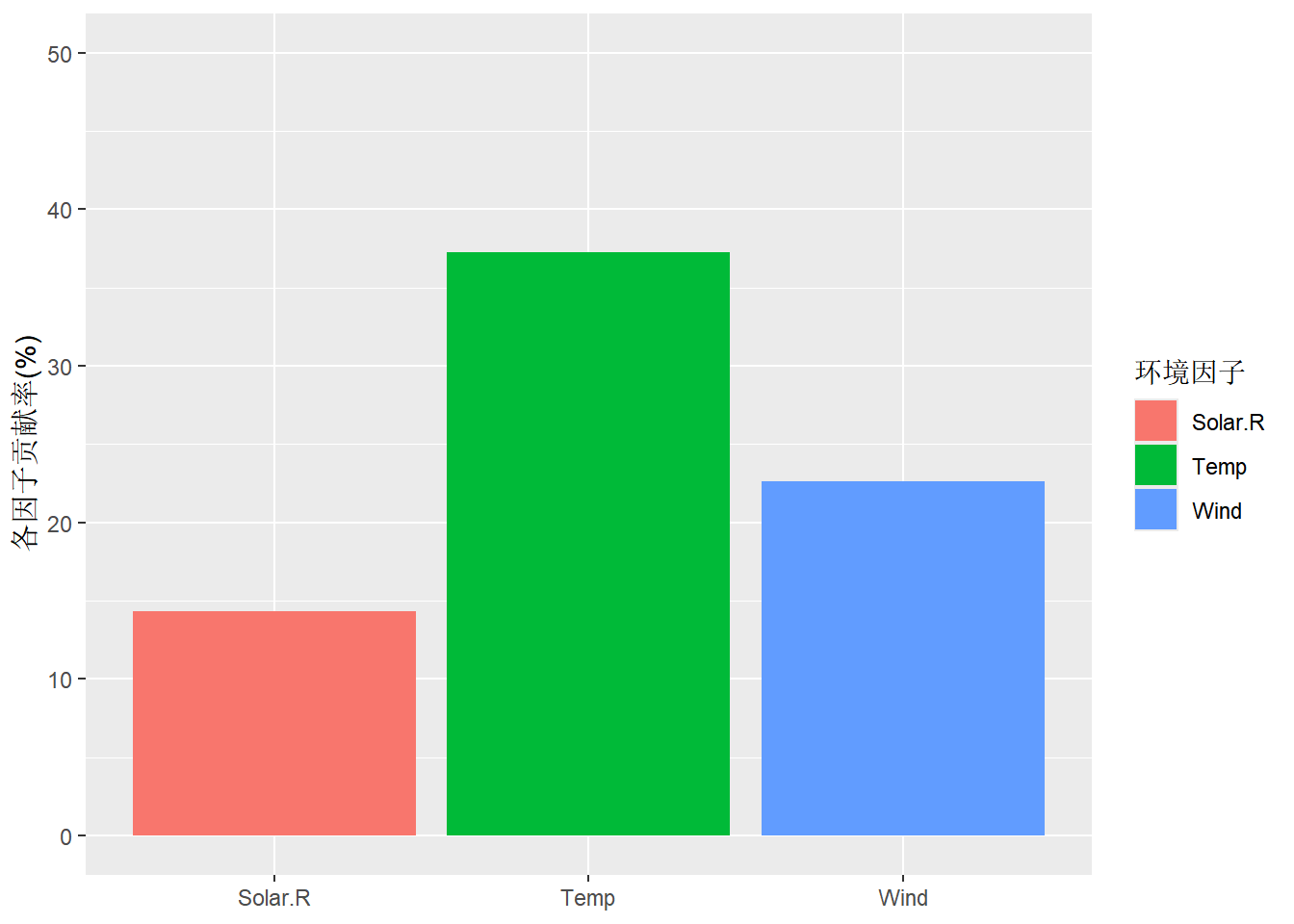
12.3.2 采用rfPermute包
rfPermute包不仅可以计算出贡献率,还可以进行显著性检测。
set.seed(20241102)
rf.2 <- rfPermute(Ozone~Solar.R+Wind+Temp,
                  data = dat,
                  importance=TRUE,
                  ntree=500,
                  nrep=100, # 设定100次随机置换
                  num.cores = 1 # 设置是否进行多线程运算
                  )
print(rf.2)
An rfPermute model
Type of random forest: regression
Number of trees: 500
No. of variables tried at each split: 1
No. of permutation replicates: 100
Start time: 2025-04-19 09:57:32
End time: 2025-04-19 09:57:37
Run time: 4.51 secs
Mean of squared residuals: 301
% Var explained: 72.5 由上述结果可知,随机森林生成了500个树,每个节点随机抽取1个变量进行模型拟合。拟合后模型可以解释72.5%的变异。
imp.2 <- importance(rf.2,scale = TRUE)
imp.2 %>% kableExtra::kable()| %IncMSE | %IncMSE.pval | IncNodePurity | IncNodePurity.pval | |
|---|---|---|---|---|
| Temp | 37.23705 | 0.009901 | 48191.67 | 0.009901 |
| Wind | 22.62814 | 0.009901 | 42588.75 | 0.009901 |
| Solar.R | 14.35751 | 0.009901 | 23417.42 | 1.000000 |
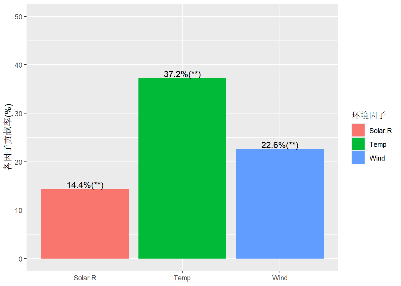
表 12.3 %IncMSE 和 IncNodePurity列为贡献率,%IncMSE.pval和IncNodePurity.pval为对应的p值,选择其一即可。 根据%IncMSE可知,Temp、Wind和Solar.R三个因子分别贡献了37.2%、22.6%和14.4%的变异,且p值均小于0.05.
imp.2 <- imp.2 %>% as.data.frame() %>% rownames_to_column(var="fct") %>%
  mutate(fct=factor(fct),
         sig=case_when(`%IncMSE.pval`<0.01~"**",
                       `%IncMSE.pval`<0.05~"*",
                       .default = ""))
ggplot(imp.2,aes(x=fct,y=`%IncMSE`,fill=fct))+
  geom_bar(stat="identity")+
  geom_text(aes(label=sprintf("%00.1f%%(%s)",`%IncMSE`,sig)),vjust = -0.2)+
  ylim(0,50)+
  labs(y="各因子贡献率(%)",x=NULL,fill="环境因子")