library(pacman)
p_load("FactoMineR","FactoMineR","tidyverse","ggrepel","latex2exp")13.1 加载工具包
13.2 加载数据集
以笔者课题组某处试验田数据为例,进行PCA分析,具体数据见表 13.1。
dt <- readxl::read_xlsx("RES/dataset/PCA.xlsx")
dt %>% knitr::kable(digits = 2)| trt | N2OEmissions | N_NH4 | N_NO3 | Eh | pH | Tem | Nuptake | Yield |
|---|---|---|---|---|---|---|---|---|
| ICFZ0 | 1.31 | 12.02 | 1.35 | 367.81 | 6.14 | 23.33 | 99.77 | 7.42 |
| ICFZ0 | 1.00 | 12.44 | 1.46 | 365.94 | 6.13 | 23.88 | 91.09 | 7.49 |
| ICFZ0 | 1.06 | 11.79 | 1.37 | 367.20 | 6.11 | 23.14 | 94.94 | 7.27 |
| IAWDZ0 | 2.84 | 12.51 | 1.36 | 406.02 | 6.21 | 23.40 | 103.36 | 7.16 |
| IAWDZ0 | 3.08 | 10.88 | 1.32 | 417.44 | 6.19 | 24.02 | 102.96 | 8.39 |
| IAWDZ0 | 2.92 | 10.18 | 1.46 | 406.64 | 6.19 | 22.98 | 92.43 | 8.09 |
| IAWDZ10 | 1.91 | 15.74 | 1.69 | 377.14 | 6.29 | 23.33 | 119.85 | 9.82 |
| IAWDZ10 | 2.07 | 15.43 | 1.59 | 389.08 | 6.26 | 24.01 | 120.78 | 8.89 |
| IAWDZ10 | 2.14 | 14.96 | 1.63 | 385.77 | 6.25 | 23.14 | 123.49 | 9.97 |
13.3 PCA 计算
利用FactoMineR包PCA函数进行PCA分析。
dt_data <- dt %>% select(-trt)
result.pca <- PCA(dt_data,graph = FALSE)
## 下面的步骤,用于对个体图坐标进行标准化
R=sum(result.pca$eig[1:2,1]^2)^0.5
result.pca$ind$coord[,1] <- result.pca$ind$coord[,1]/R
result.pca$ind$coord[,2] <- result.pca$ind$coord[,2]/R
13.4 绘图
主要包括变量图和个体图两个数据集
13.4.1 变量图数据准备
variables <- result.pca$var$coord %>%
  as.data.frame() %>%
  tibble::rownames_to_column(var = "response") %>%
  select(response,Dim.1, Dim.2)
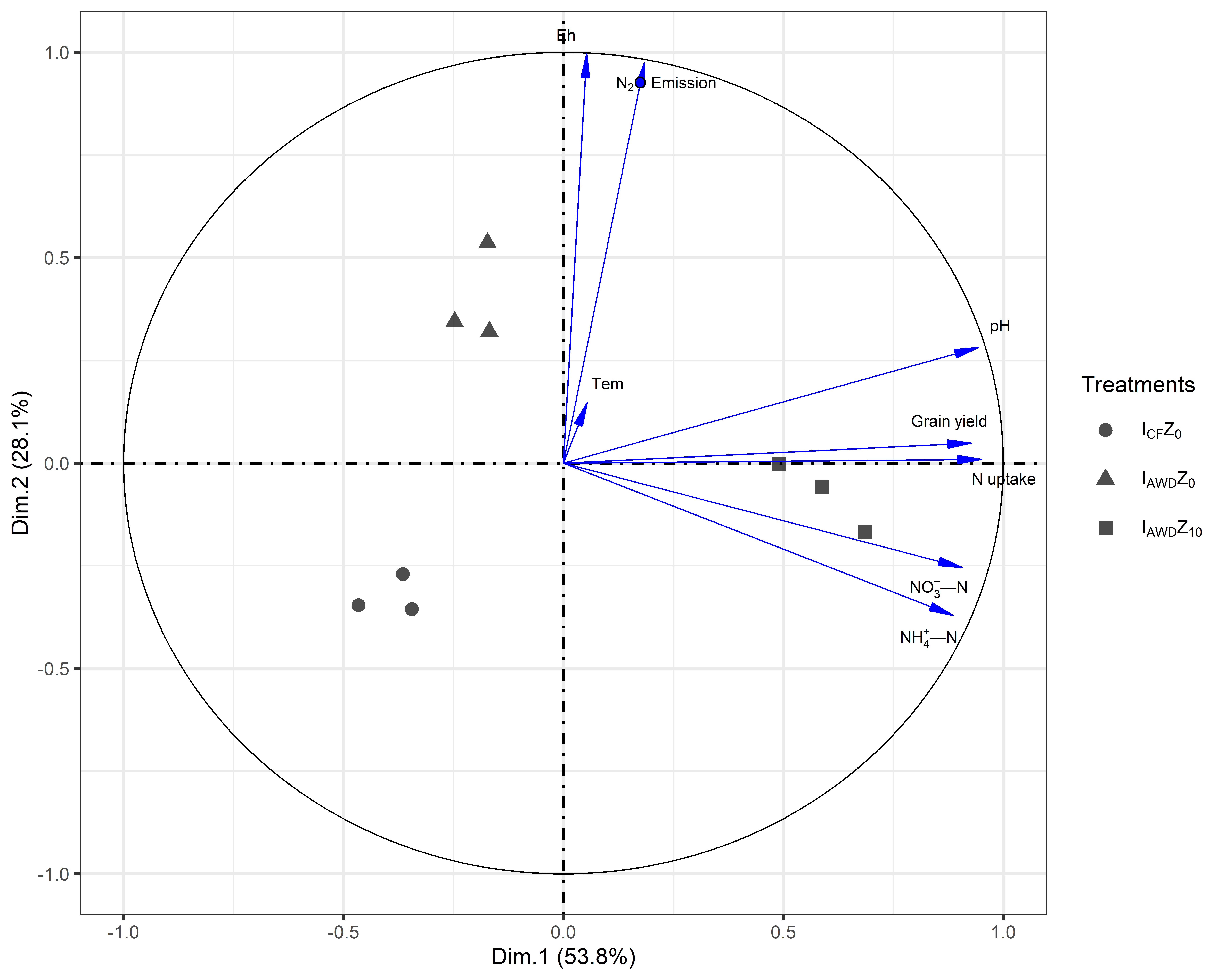
variables %>% knitr::kable(digits = 2)| response | Dim.1 | Dim.2 |
|---|---|---|
| N2OEmissions | 0.18 | 0.97 |
| N_NH4 | 0.89 | -0.37 |
| N_NO3 | 0.91 | -0.25 |
| Eh | 0.05 | 1.00 |
| pH | 0.94 | 0.28 |
| Tem | 0.05 | 0.15 |
| Nuptake | 0.95 | 0.01 |
| Yield | 0.93 | 0.05 |
13.4.2 个体图数据准备
TrtPoints <-  result.pca$ind$coord %>%
  as.data.frame() %>%
  mutate(trt=dt$trt) %>%
  select(trt, Dim.1, Dim.2) %>%
  mutate(trt=factor(trt,levels=c("ICFZ0","IAWDZ0","IAWDZ10")))
TrtPoints %>% knitr::kable(digits = 2)| trt | Dim.1 | Dim.2 |
|---|---|---|
| ICFZ0 | -0.36 | -0.27 |
| ICFZ0 | -0.34 | -0.36 |
| ICFZ0 | -0.47 | -0.35 |
| IAWDZ0 | -0.17 | 0.32 |
| IAWDZ0 | -0.17 | 0.54 |
| IAWDZ0 | -0.25 | 0.34 |
| IAWDZ10 | 0.69 | -0.17 |
| IAWDZ10 | 0.49 | 0.00 |
| IAWDZ10 | 0.59 | -0.06 |
13.4.3 重定义标签
responselabels <- c(
  TeX("$N_{2}O$ Emission"),
  TeX("$NH_{4}^{+}$—N"),
  TeX("$NO_{3}^{-}$—N"),
  "Eh",
  "pH",
  "Tem",
  "N~uptake",
  "Grain~yield"
)
13.4.4 ggplot绘图
lab1 <- c(  expression(I[CF]*Z[0]),  expression(I[AWD]*Z[0]),  expression(I[AWD]*Z[10]))

G <- ggplot(variables, aes(x = Dim.1, y = Dim.2)) +
  annotate("path",
           x = cos(seq(0, 2 * pi, length.out = 200)),
           y = sin(seq(0, 2 * pi, length.out = 200)),
           linewidth = 0.25) +
  geom_hline(yintercept = 0, linetype = 4) +
  geom_vline(xintercept = 0, linetype = 4) +
  geom_point(
    data = TrtPoints,
    aes(x = Dim.1, y = Dim.2, shape = trt),
    size = 2,
    alpha = 0.7
  ) +
  scale_shape_discrete(labels = lab1) +
  geom_segment(
    aes(
      x = 0,
      y = 0,
      xend = Dim.1,
      yend = Dim.2
    ),
    color = "blue",
    linewidth = 0.25,
    arrow = arrow(
      angle = 10,
      length = unit(0.3, "cm"),
      type = "closed"
    )
  ) +
  geom_text_repel(label=responselabels,parse=TRUE,size=2)+
  labs(shape="Treatments",x=sprintf("Dim.1 (%.1f%%)",result.pca$eig[1,2]),
       y=sprintf("Dim.2 (%.1f%%)",result.pca$eig[2,2]))+
  theme_bw(base_line_size = 0.5,base_size = 8)

G