library(lavaan)
library(tidyverse)
library(tidySEM)
library(semPlot)15.1 加载工具包
这是一个研究学生的学业成绩影响因素的研究,主要包括9个观测指标(9个变量):Motivation(动机), Harmony(和谐), Stability(稳定), Negative Parental Psychology(消极的父母心理), SES, Verbal IQ(语言智力), Reading(阅读), Arithmetic (算术)and Spelling(拼写)。研究员假设三个潜变量:Adjustment(自我调节), Risk(抗风险), Achievement(未来成就), 他们的测量指标如下, 其中包含了变量名及其解释:
- Adjustment(自我调节)
- motiv Motivation
- harm Harmony
- stabi Stability
- Risk
- ppsych (Negative) Parental Psychology
- ses SES
- verbal Verbal IQ
- Achievement
- read Reading
- arith Arithmetic
- spell Spelling
15.2 读取数据集
数据集网址为https://stats.idre.ucla.edu/wp-content/uploads/2021/02/worland5.csv,可以用R直接读取。前20行间表
dat <- read.csv("https://stats.idre.ucla.edu/wp-content/uploads/2021/02/worland5.csv")
dat %>% head(20)| motiv | harm | stabi | ppsych | ses | verbal | read | arith | spell |
|---|---|---|---|---|---|---|---|---|
| -7.907122 | -5.075312 | -3.138836 | -17.800210 | 4.766450 | -3.633360 | -3.488981 | -9.989121 | -6.567873 |
| 1.751478 | -4.155847 | 3.520752 | 7.009367 | -6.048681 | -7.693461 | -4.520552 | 8.196238 | 8.778973 |
| 14.472570 | -4.540677 | 4.070600 | 23.734260 | -16.970670 | -3.909941 | -4.818170 | 7.529984 | -5.688716 |
| -1.165421 | -5.668406 | 2.600437 | 1.493158 | 1.396363 | 21.409450 | -3.138441 | 5.730547 | -2.915676 |
| -4.222899 | -10.072150 | -6.030737 | -5.985864 | -18.376400 | -1.438816 | -2.009742 | -0.623953 | -1.024624 |
| 4.868769 | 3.029841 | -7.648277 | 14.668790 | -2.235039 | -6.826892 | 0.822650 | 5.045174 | 0.904154 |
| 10.367370 | 5.039368 | 6.031902 | -0.952449 | -9.258073 | 8.485556 | -5.672760 | 8.638372 | -1.525859 |
| -1.861007 | 0.398970 | -1.041958 | -14.569340 | -15.998880 | -0.763939 | -11.338880 | 3.753714 | -7.449076 |
| -13.452220 | -15.333230 | -10.938220 | -5.084801 | -3.269256 | -1.157033 | 2.397864 | -8.260820 | 2.343741 |
| 2.852636 | 2.202829 | -3.961495 | 11.203110 | 0.255099 | -11.238150 | -5.819805 | -1.407573 | -2.550445 |
| -2.135480 | -4.988594 | -5.197804 | 18.165050 | -8.722278 | -22.846290 | -9.586946 | -5.120381 | -10.116000 |
| -13.271710 | -14.716500 | -22.237840 | -13.617300 | -2.468196 | 3.227680 | -3.136714 | -9.810998 | -5.178977 |
| 0.074682 | -3.900125 | -0.681536 | 13.456060 | -1.117470 | -3.047351 | -11.526480 | -5.075179 | 1.392740 |
| -1.234672 | -7.602469 | -11.120770 | 9.088286 | -8.614449 | -2.908931 | -0.894078 | 3.111883 | 4.711888 |
| 16.215860 | 9.221498 | 6.272686 | 7.127136 | 4.019466 | 6.209437 | -3.797352 | 2.665741 | -2.957346 |
| 2.627465 | 12.146830 | 13.391960 | -8.771418 | 7.053579 | 7.898940 | 0.989484 | -5.955518 | -0.981625 |
| -20.947040 | -24.684320 | -4.687459 | 12.434270 | -1.293421 | 2.824059 | -9.806948 | -9.956636 | -15.627680 |
| 1.803133 | -12.255210 | -1.746126 | -20.890180 | -4.172909 | 8.513219 | 8.840849 | 1.007681 | -1.835484 |
| -2.228813 | -4.254879 | 12.911310 | 16.996250 | -0.283493 | -8.754460 | -12.233980 | -2.866628 | -19.672850 |
| 14.554980 | 18.997670 | 3.717919 | -3.370208 | 13.400550 | 12.263600 | 12.793220 | 14.937080 | 14.768940 |
15.3 构建结构方程模型
15.3.1 构建结构方程模型
m6b1 <- '
# measurement model  定义潜变量,设置测量模型
adjust =~ motiv + harm + stabi
risk =~ verbal + ses + ppsych
achieve =~ read + arith + spell
# regressions 回归模型
adjust ~ risk
achieve ~ adjust + risk
'
fit6b <- sem(m6b1, data = dat)
result <- summary(fit6b, standardized = TRUE, fit.measures = TRUE)
result
lavaan 0.6-19 ended normally after 112 iterations
Estimator ML
Optimization method NLMINB
Number of model parameters 21
Number of observations 500
Model Test User Model:
Test statistic 148.982
Degrees of freedom 24
P-value (Chi-square) 0.000
Model Test Baseline Model:
Test statistic 2597.972
Degrees of freedom 36
P-value 0.000
User Model versus Baseline Model:
Comparative Fit Index (CFI) 0.951
Tucker-Lewis Index (TLI) 0.927
Loglikelihood and Information Criteria:
Loglikelihood user model (H0) -15517.857
Loglikelihood unrestricted model (H1) -15443.366
Akaike (AIC) 31077.713
Bayesian (BIC) 31166.220
Sample-size adjusted Bayesian (SABIC) 31099.565
Root Mean Square Error of Approximation:
RMSEA 0.102
90 Percent confidence interval - lower 0.087
90 Percent confidence interval - upper 0.118
P-value H_0: RMSEA <= 0.050 0.000
P-value H_0: RMSEA >= 0.080 0.990
Standardized Root Mean Square Residual:
SRMR 0.041
Parameter Estimates:
Standard errors Standard
Information Expected
Information saturated (h1) model Structured
Latent Variables:
Estimate Std.Err z-value P(>|z|) Std.lv Std.all
adjust =~
motiv 1.000 9.324 0.933
harm 0.884 0.041 21.774 0.000 8.246 0.825
stabi 0.695 0.043 15.987 0.000 6.478 0.648
risk =~
verbal 1.000 7.319 0.733
ses 0.807 0.076 10.607 0.000 5.906 0.591
ppsych -0.770 0.075 -10.223 0.000 -5.636 -0.564
achieve =~
read 1.000 9.404 0.941
arith 0.837 0.034 24.437 0.000 7.873 0.788
spell 0.976 0.028 34.338 0.000 9.178 0.919
Regressions:
Estimate Std.Err z-value P(>|z|) Std.lv Std.all
adjust ~
risk 0.599 0.076 7.837 0.000 0.470 0.470
achieve ~
adjust 0.375 0.046 8.085 0.000 0.372 0.372
risk 0.724 0.078 9.253 0.000 0.564 0.564
Variances:
Estimate Std.Err z-value P(>|z|) Std.lv Std.all
.motiv 12.870 2.852 4.512 0.000 12.870 0.129
.harm 31.805 2.973 10.698 0.000 31.805 0.319
.stabi 57.836 3.990 14.494 0.000 57.836 0.580
.verbal 46.239 4.788 9.658 0.000 46.239 0.463
.ses 64.916 4.975 13.048 0.000 64.916 0.650
.ppsych 68.033 5.068 13.425 0.000 68.033 0.682
.read 11.372 1.608 7.074 0.000 11.372 0.114
.arith 37.818 2.680 14.109 0.000 37.818 0.379
.spell 15.560 1.699 9.160 0.000 15.560 0.156
.adjust 67.694 6.066 11.160 0.000 0.779 0.779
risk 53.561 6.757 7.927 0.000 1.000 1.000
.achieve 30.685 3.449 8.896 0.000 0.347 0.34715.3.2 输出结构方程模型参数
result$pe| lhs | op | rhs | exo | est | se | z | pvalue | std.lv | std.all |
|---|---|---|---|---|---|---|---|---|---|
| adjust | =~ | motiv | 0 | 1.0000000 | 0.0000000 | NA | NA | 9.3236112 | 0.9332948 |
| adjust | =~ | harm | 0 | 0.8844138 | 0.0406182 | 21.773843 | 0.0e+00 | 8.2459306 | 0.8254189 |
| adjust | =~ | stabi | 0 | 0.6947893 | 0.0434593 | 15.987116 | 0.0e+00 | 6.4779457 | 0.6484433 |
| risk | =~ | verbal | 0 | 1.0000000 | 0.0000000 | NA | NA | 7.3185705 | 0.7325900 |
| risk | =~ | ses | 0 | 0.8070235 | 0.0760846 | 10.606927 | 0.0e+00 | 5.9062586 | 0.5912174 |
| risk | =~ | ppsych | 0 | -0.7701249 | 0.0753298 | -10.223381 | 0.0e+00 | -5.6362132 | -0.5641858 |
| achieve | =~ | read | 0 | 1.0000000 | 0.0000000 | NA | NA | 9.4035951 | 0.9413013 |
| achieve | =~ | arith | 0 | 0.8372176 | 0.0342603 | 24.436932 | 0.0e+00 | 7.8728550 | 0.7880740 |
| achieve | =~ | spell | 0 | 0.9760348 | 0.0284241 | 34.338325 | 0.0e+00 | 9.1782364 | 0.9187428 |
| adjust | ~ | risk | 0 | 0.5992803 | 0.0764724 | 7.836560 | 0.0e+00 | 0.4704052 | 0.4704052 |
| achieve | ~ | adjust | 0 | 0.3747906 | 0.0463570 | 8.084875 | 0.0e+00 | 0.3716028 | 0.3716028 |
| achieve | ~ | risk | 0 | 0.7243599 | 0.0782844 | 9.252929 | 0.0e+00 | 0.5637503 | 0.5637503 |
| motiv | ~~ | motiv | 0 | 12.8702817 | 2.8522325 | 4.512354 | 6.4e-06 | 12.8702817 | 0.1289607 |
| harm | ~~ | harm | 0 | 31.8046281 | 2.9729464 | 10.698016 | 0.0e+00 | 31.8046281 | 0.3186837 |
| stabi | ~~ | stabi | 0 | 57.8362265 | 3.9902389 | 14.494427 | 0.0e+00 | 57.8362265 | 0.5795213 |
| verbal | ~~ | verbal | 0 | 46.2385229 | 4.7877650 | 9.657643 | 0.0e+00 | 46.2385229 | 0.4633119 |
| ses | ~~ | ses | 0 | 64.9161012 | 4.9752240 | 13.047875 | 0.0e+00 | 64.9161012 | 0.6504620 |
| ppsych | ~~ | ppsych | 0 | 68.0331022 | 5.0675179 | 13.425330 | 0.0e+00 | 68.0331022 | 0.6816944 |
| read | ~~ | read | 0 | 11.3724048 | 1.6076452 | 7.073952 | 0.0e+00 | 11.3724048 | 0.1139519 |
| arith | ~~ | arith | 0 | 37.8181571 | 2.6804197 | 14.109043 | 0.0e+00 | 37.8181571 | 0.3789394 |
| spell | ~~ | spell | 0 | 15.5599796 | 1.6986471 | 9.160219 | 0.0e+00 | 15.5599796 | 0.1559116 |
| adjust | ~~ | adjust | 0 | 67.6938212 | 6.0658595 | 11.159807 | 0.0e+00 | 0.7787189 | 0.7787189 |
| risk | ~~ | risk | 0 | 53.5614747 | 6.7571328 | 7.926657 | 0.0e+00 | 1.0000000 | 1.0000000 |
| achieve | ~~ | achieve | 0 | 30.6848664 | 3.4494126 | 8.895679 | 0.0e+00 | 0.3470055 | 0.3470055 |
15.3.3 结构方程模型出图
semPlot::semPaths(fit6b, 'std',layout="spring")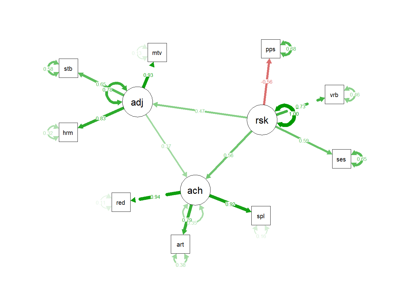
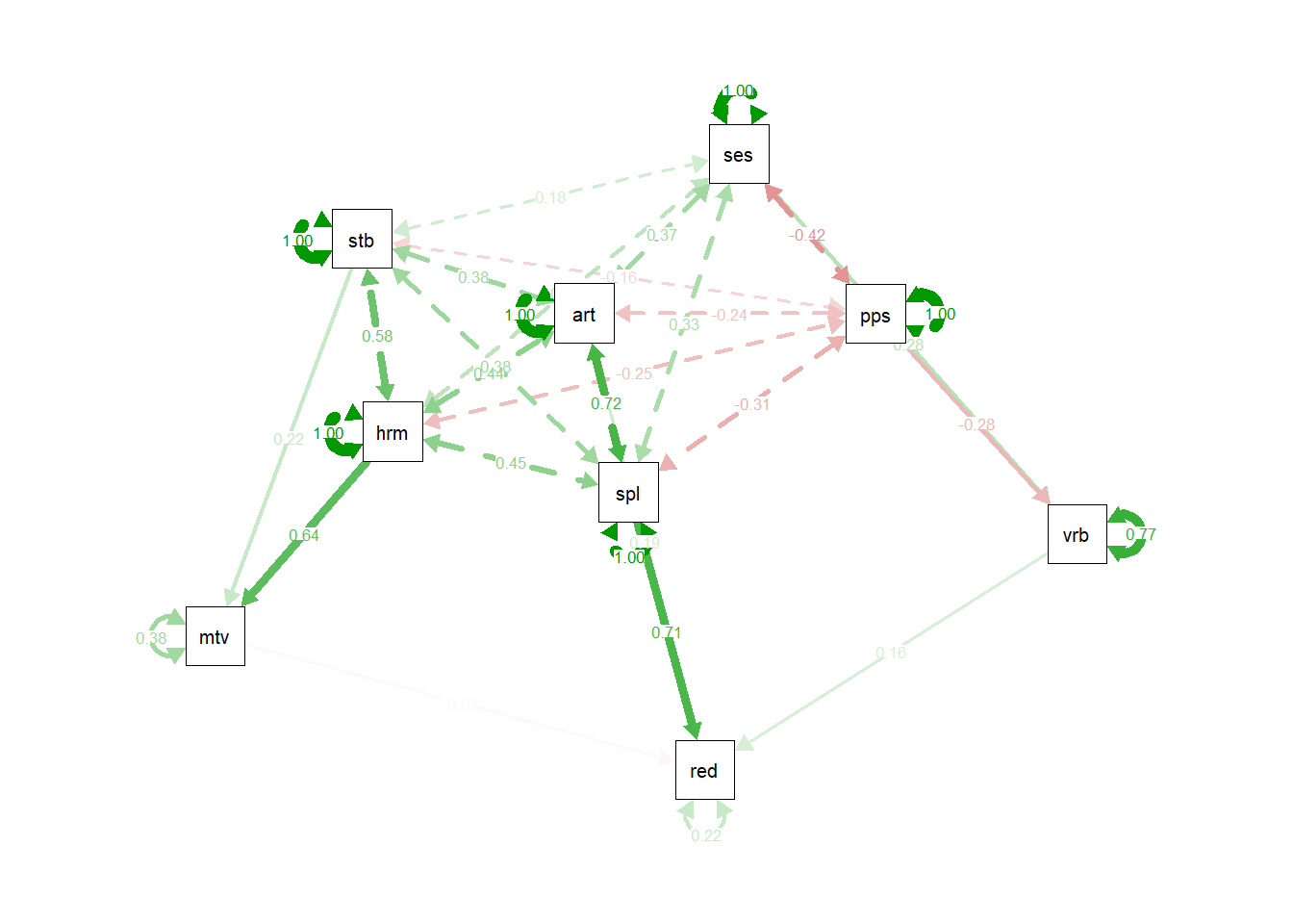
有些学者可能更偏向于不设置潜在变量,所有变量都是观测变量,也可不设置潜变量,直接用结构模型
m6b2 <- '
# measurement model
motiv~ harm + stabi
verbal ~ ses + ppsych
read ~ arith + spell
# regressions
read~ motiv+ verbal
'
fit6b <- sem(m6b2, data = dat)
result <- summary(fit6b, standardized = TRUE, fit.measures = TRUE)
result$pe| lhs | op | rhs | exo | est | se | z | pvalue | std.lv | std.all | std.nox |
|---|---|---|---|---|---|---|---|---|---|---|
| motiv | ~ | harm | 0 | 0.6446655 | 0.0336682 | 19.147583 | 0.0000000 | 0.6446655 | 0.6446655 | 0.0645311 |
| motiv | ~ | stabi | 0 | 0.2160940 | 0.0336682 | 6.418334 | 0.0000000 | 0.2160940 | 0.2160940 | 0.0216310 |
| verbal | ~ | ses | 0 | 0.2816901 | 0.0433720 | 6.494753 | 0.0000000 | 0.2816901 | 0.2816901 | 0.0281972 |
| verbal | ~ | ppsych | 0 | -0.2816901 | 0.0433720 | -6.494753 | 0.0000000 | -0.2816901 | -0.2816901 | -0.0281972 |
| read | ~ | arith | 0 | 0.1808558 | 0.0294307 | 6.145141 | 0.0000000 | 0.1808558 | 0.1871507 | 0.0187338 |
| read | ~ | spell | 0 | 0.6851775 | 0.0295503 | 23.186831 | 0.0000000 | 0.6851775 | 0.7090259 | 0.0709736 |
| read | ~ | motiv | 0 | -0.0316029 | 0.0219917 | -1.437035 | 0.1507079 | -0.0316029 | -0.0327029 | -0.0327029 |
| read | ~ | verbal | 0 | 0.1526084 | 0.0205501 | 7.426168 | 0.0000000 | 0.1526084 | 0.1579201 | 0.1579201 |
| motiv | ~~ | motiv | 0 | 37.5359884 | 2.3739844 | 15.811388 | 0.0000000 | 37.5359884 | 0.3761121 | 0.3761121 |
| verbal | ~~ | verbal | 0 | 77.3098585 | 4.8895048 | 15.811388 | 0.0000000 | 77.3098585 | 0.7746479 | 0.7746479 |
| read | ~~ | read | 0 | 20.2753349 | 1.2823248 | 15.811388 | 0.0000000 | 20.2753349 | 0.2175482 | 0.2175482 |
| harm | ~~ | harm | 1 | 99.7999994 | 0.0000000 | NA | NA | 99.7999994 | 1.0000000 | 99.7999994 |
| harm | ~~ | stabi | 1 | 57.8840009 | 0.0000000 | NA | NA | 57.8840009 | 0.5800000 | 57.8840009 |
| harm | ~~ | ses | 1 | 25.9479982 | 0.0000000 | NA | NA | 25.9479982 | 0.2600000 | 25.9479982 |
| harm | ~~ | ppsych | 1 | -24.9499985 | 0.0000000 | NA | NA | -24.9499985 | -0.2500000 | -24.9499985 |
| harm | ~~ | arith | 1 | 43.9120006 | 0.0000000 | NA | NA | 43.9120006 | 0.4400000 | 43.9120006 |
| harm | ~~ | spell | 1 | 44.9100004 | 0.0000000 | NA | NA | 44.9100004 | 0.4500000 | 44.9100004 |
| stabi | ~~ | stabi | 1 | 99.8000037 | 0.0000000 | NA | NA | 99.8000037 | 1.0000000 | 99.8000037 |
| stabi | ~~ | ses | 1 | 17.9639995 | 0.0000000 | NA | NA | 17.9639995 | 0.1800000 | 17.9639995 |
| stabi | ~~ | ppsych | 1 | -15.9679995 | 0.0000000 | NA | NA | -15.9679995 | -0.1600000 | -15.9679995 |
| stabi | ~~ | arith | 1 | 37.9240014 | 0.0000000 | NA | NA | 37.9240014 | 0.3800000 | 37.9240014 |
| stabi | ~~ | spell | 1 | 37.9240037 | 0.0000000 | NA | NA | 37.9240037 | 0.3800000 | 37.9240037 |
| ses | ~~ | ses | 1 | 99.7999978 | 0.0000000 | NA | NA | 99.7999978 | 1.0000000 | 99.7999978 |
| ses | ~~ | ppsych | 1 | -41.9159985 | 0.0000000 | NA | NA | -41.9159985 | -0.4200000 | -41.9159985 |
| ses | ~~ | arith | 1 | 36.9259979 | 0.0000000 | NA | NA | 36.9259979 | 0.3700000 | 36.9259979 |
| ses | ~~ | spell | 1 | 32.9339995 | 0.0000000 | NA | NA | 32.9339995 | 0.3300000 | 32.9339995 |
| ppsych | ~~ | ppsych | 1 | 99.7999951 | 0.0000000 | NA | NA | 99.7999951 | 1.0000000 | 99.7999951 |
| ppsych | ~~ | arith | 1 | -23.9520005 | 0.0000000 | NA | NA | -23.9520005 | -0.2400000 | -23.9520005 |
| ppsych | ~~ | spell | 1 | -30.9379995 | 0.0000000 | NA | NA | -30.9379995 | -0.3100000 | -30.9379995 |
| arith | ~~ | arith | 1 | 99.8000018 | 0.0000000 | NA | NA | 99.8000018 | 1.0000000 | 99.8000018 |
| arith | ~~ | spell | 1 | 71.8560021 | 0.0000000 | NA | NA | 71.8560021 | 0.7200000 | 71.8560021 |
| spell | ~~ | spell | 1 | 99.7999997 | 0.0000000 | NA | NA | 99.7999997 | 1.0000000 | 99.7999997 |
semPlot::semPaths(fit6b, 'std',layout="spring")